
When I first studied production theory in college, I struggled to picture how a firm balances labor and capital to keep output steady until I sketched my first isoquant curve on paper.
The word itself comes from mixing a Greek word, “is,” with a Latin word, “quant,” and together they simply mean equal quantity or equal product.
That is why economists also call it the equal product curve, a curve representation of every inputs combination a producer can use to reach the same output level.
[INTERNAL LINK OPPORTUNITY: link “production theory” or “microeconomics” to a related economics/basics-of-economics article on your site, if you have one]
In microeconomics, the isoquant works almost like a firm’s counterpart of a household budget line, except here it mirrors the consumer’s indifference curve which is why it also earns the nickname producer’s indifference curve.
Along any single curve, a producer stays indifferent between different combinations of two inputs, because every point sits on the same product level.
This graphical representation traces the locus of points where the relationship between inputs never changes the final same level of output.
Studying the behavior of producers taught me that businesses rarely fix their production processes to one rigid method; instead, they shift between combinations to optimize costs.
Grasping the properties of isoquants becomes a fundamental concept for any student of production functions, because it shows exactly how businesses try to maximize profits while keeping production efficient, since every input change carries a direct effect on output.
Properties of Isoquant
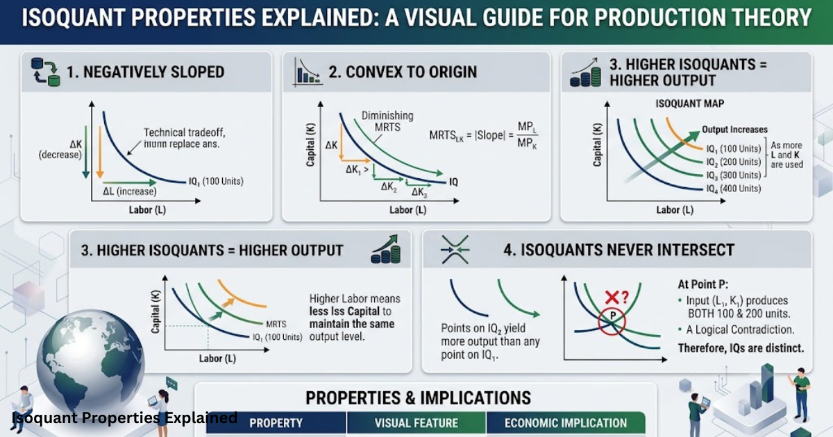
Every isoquant curve is negatively sloped, running from left to right in a way that looks downward sloping on the graph, and the slope itself tells a real story about the trade-off between inputs.
To keep output constant, a firm cannot add more of one input without giving up capital somewhere else that constant back-and-forth is what economists call substitution of inputs, guided by the rate of substitution between labor and machines.
I’ve noticed that a curve sitting further from the origin always signals higher production; a higher isoquant stands for higher output, while a curve closer in reflects lower output and a lower isoquant.
Two isoquants can never cross, because non-intersecting curves protect the idea that two isoquants cannot share a point without contradicting each other’s different levels of output and that is also why curves stay away from zero inputs, refusing to touch the origin, since no factory can produce anything from nothing.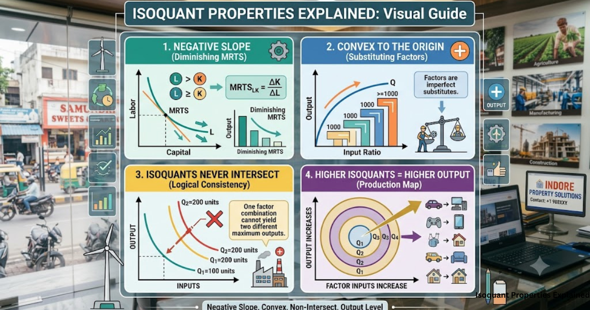 Curves also bend convex to the origin rather than concave to the origin, because the marginal rate of technical substitution often shortened to MRTS keeps falling as increasing labor replaces machines; that steady diminishing pattern reflects technical substitution at work.
Similar to how adding more workers to a factory creates overcrowding and a diminishing marginal product, each extra hand adds less to the marginal product overall.
Two curves can only run as parallel curves when their input combinations share an equal MRTS, and this behaviour stays realistic because economists assume no kinks or discontinuities break the line.
Instead, the shape stays smooth and continuous, showing smoothness and a continuous substitution even through small changes or large changes in large scale production, always following the same combination of inputs logic that keeps a firm’s curves from ever managing to intersect.
Few Definitions of Isoquant Curve
Every solid definition of this curve traces back to a handful of classic economists. Bilas described isoproduct curves as the way a firm shows every combination of two resources that can produce an equal amount of product. Samuelson kept it simple by saying the curve shows the input combinations that reach a given output.
Isoquant Properties Explained it as the possible combinations of two variable factors used to make the same total product, and Ferguson went further, calling it every combination physically capable of reaching a given level of output.
Example of Isoquant Schedule and Isoquant Curve
A simple isoquant schedule makes all this easier to picture. Imagine a table listing five combinations: in combination A, a firm uses 1 unit of labor (L) and 12 units of capital (K) to reach 100 units of output. Combination B swaps in 2 labor for 8 capital; combination C moves to 3 labor and 5 capital. Combination D shifts to 4 labor and 3 capital, and combination E reaches 5 labor with just 2 capital. Every row still lands on the same output units, and plotting this data on a figure gives the familiar graphical representation of the curve.
Assumptions of Isoquant Curve
Production theory hold this whole model together. First, only labor and capital enter the production process, and the production function follows a variable proportion shape, meaning there is real technical possibility for substituting inputs freely. Second, both inputs stay divisible, so a firm can adjust them in small steps.
Third, we assume a rational producer who always works to maximize profit, operating under an unchanged technology in other words, the state of technology stays fixed while the diminishing MRTS rule keeps guiding how two inputs trade off against each other.
Marginal Rate of Technical Substitution
The marginal rate of technical substitution, or MRTS, measures exactly how many units of capital a firm gives up for each extra units of labor, while producing the same commodity.
Moving from combination A to combination B trades away capital at a 4:1 ratio; from combination B to combination C, the swap slows to 3:1.
From combination microeconomics D, it drops to 2:1; and from combination D to combination E, the rate settles at 1:1. This whole pattern of labor for capital shows a factor substitution that keeps the output level and output constant the entire time, and at any point on curve, you can find the exact slope by drawing a tangent line a neat mathematical representation of the production process that links labor L and capital K together.
FAQs About Isoquant Properties Explained
What are the main properties of an isoquant?
An isoquant is negatively sloped, stays convex to the origin, and never lets two isoquants cross, since non-intersecting curves protect each output level.
Why is an isoquant convex to the origin?
Because the marginal rate of technical substitution keeps diminishing — as a firm keeps increasing labor, it gives up smaller amounts of capital each time, which naturally bends the curve convex to the origin.
Can two isoquants intersect each other?
No. If two isoquants could intersect, the same input combinations would show two different levels of output, which breaks the logic of a production function entirely.
What does MRTS mean in isoquant analysis?
MRTS stands for the marginal rate of technical substitution it shows how many units of capital a firm trades for extra units of labor while keeping the output constant.
Why does an isoquant never touch the axes?
Because production needs both inputs together; with zero inputs on either side, a factory simply cannot touch the origin and still generate any output.